
ggplot basics
Published:
Generate a volcano plot using ggplot2!
Introduction
This document demonstrates how to generate a volcano plot using ggplot2 by reading a CSV file that contains gene expression data. The dataset must include at least three mandatory columns:
log2FC(Log2 Fold Change)p_value(P-value for statistical significance)Gene_symbol(or Gene EntrezID or Gene ENSEMBL ID)
Each step is explained in detail, with code chunks for clarity.
Installing and Loading Required Libraries
Check if required packages are installed, if not install them
    if (!requireNamespace("ggplot2", quietly = TRUE)) {
      install.packages("ggplot2")
    }

    if (!requireNamespace("ggrepel", quietly = TRUE)) {
      install.packages("ggrepel")
    }

    if (!requireNamespace("dplyr", quietly = TRUE)) {
      install.packages("dplyr")
    }
Load libraries
    library(ggplot2)

    ## RStudio Community is a great place to get help:
    ## https://community.rstudio.com/c/tidyverse

    library(dplyr)

    ##
    ## Attaching package: 'dplyr'

    ## The following objects are masked from 'package:stats':
    ##
    ##     filter, lag

    ## The following objects are masked from 'package:base':
    ##
    ##     intersect, setdiff, setequal, union

    library(ggrepel)
Setting Up Project Directories
    project_dir <- "/Users/debojyoti/Projects/ggplot_basics"
    data_dir <- paste0(project_dir, "/input_data")
    result_dir <- paste0(project_dir, "/results")
Create directories if they don’t exist
if (!dir.exists(result_dir)) dir.create(result_dir, recursive = TRUE)
Reading the Input Data
    input_file <- paste0(data_dir, "/test_input_file.csv")
    data <- read.csv(input_file)
Display first few rows of the dataset
    head(data)

    ##   Gene_symbol    log2FC neg_log10pval log2FC_sq      p_value
    ## 1       Gene7  2.267283     1.7250171  5.140572 0.0188357482
    ## 2       Gene9  3.027636     3.8045651  9.166577 0.0001568321
    ## 3      Gene11  1.957304     0.2616621  3.831041 0.5474417710
    ## 4      Gene12  3.429968     3.7879732 11.764681 0.0001629396
    ## 5      Gene13 -2.083291     3.8993947  4.340102 0.0001260681
    ## 6      Gene18 -3.984683     3.9222951 15.877700 0.0001195928
Transforming Data for Visualization
Before plotting, we transform the data: - Convert the p_value column to -log10(p_value) to emphasize small p-values. - Define upregulated and downregulated genes based on cutoff values. - Reverse the log2FC values for visualization.
We define thresholds for classification: - p_value cutoff: 0.05 - log2FC cutoff: 1
Define cutoffs
    pval_cutoff <- 0.05
    log2fc_cutoff <- 1
Classify genes into upregulated, downregulated, or Non-significant
    data <- data %>%
      mutate(
        logP = -log10(p_value),
        negLog2FC = -log2FC,
        regulation = case_when(
          p_value < pval_cutoff & negLog2FC > log2fc_cutoff ~ "Upregulated",
          p_value < pval_cutoff & negLog2FC < -log2fc_cutoff ~ "Downregulated",
          TRUE ~ "Non-significant"
        )
      )
Selecting Top Genes for Labeling
To highlight important genes, we select the top n genes from the upregulated and downregulated groups.
    top_n <- 5  # Number of genes to label

    top_up <- data %>%
      filter(regulation == "Upregulated") %>%
      arrange(log2FC) %>%
      head(top_n)

    top_down <- data %>%
      filter(regulation == "Downregulated") %>%
      arrange(desc(abs(log2FC))) %>%
      head(top_n)

    # Combine top genes
    top_genes <- bind_rows(top_up, top_down)
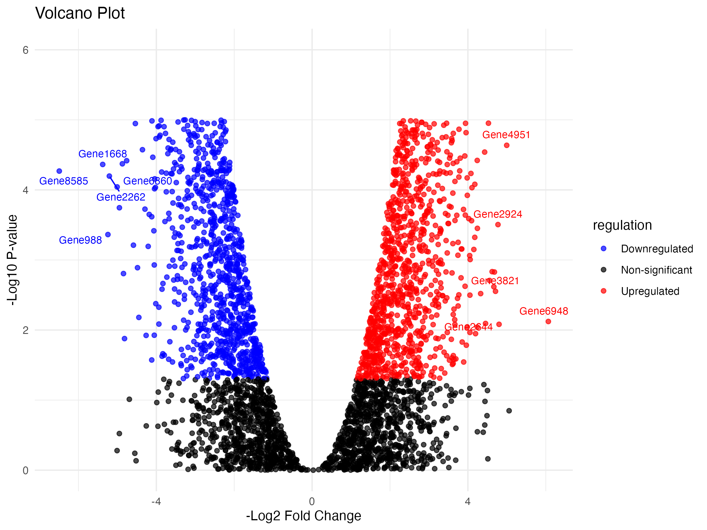
Creating the Volcano Plot
We use ggplot2 to create a volcano plot with color distinctions:
    volcano <- ggplot(data, aes(x = negLog2FC, y = logP, color = regulation)) +
      geom_point(alpha = 0.7) +
      scale_color_manual(values = c("Non-significant" = "black", "Upregulated" = "red", "Downregulated" = "blue")) +
      labs(title = "Volcano Plot", x = "-Log2 Fold Change", y = "-Log10 P-value") +
      theme_minimal() +
      geom_text_repel(
        data = top_genes,
        aes(label = Gene_symbol),
        vjust = -1,
        size = 3,
        show.legend = FALSE
        ) +
      ylim(c(0,6))
Display plot
print(volcano)
Saving the Plot
    output_file <- paste0(result_dir, "/volcano_plot.png")
    ggsave(output_file, plot = volcano, width = 8, height = 6)
Conclusion
This document demonstrated how to load, process, and visualize gene expression data using a volcano plot. We added classification for upregulated and downregulated genes, highlighted top genes, and saved the final plot.